Study

[CV][4주차_심화과제_1] CNN-Visualization

CNN-Visualization

Published 2025.09.25 Reading 8 minute read

심화_1:CNN-Visualization

CNN Visualization 방법을 구현해보기

VGG-11을 이용해서 CNN의 동작과 학습원리에 대한 직관갖기

gradient정보가 포함하고 있는 의미를 이해하고, 분석해서 활용
모델 디버깅에 필요한 기본 방법들 숙지하기
PreTrain된 모델을 분석하는 방법, 조작하는 방법에 대해 익히기

파이토치의 자동미분

파이토치는 autograd 를 통해 자동 미분을 한다. Tensor에서 requires_grad = True 옵션을 주면 파이토치는 Tensor의 연산을 추적해서 Computational Graph 를 만든다. → 이 그래프를 저장해서 Gradient를 자동으로 계산한다.

backward() 를 호출하면 만들어둔 Graph를 거꾸로 올라가며 파라미터에 대한 기울기를 자동으로 계산한다.

.backward() 가 실행된 후 requires_grad = True 로 설정했던 각 Tensor의 grad 속성(attribute)에 계산된 기울기값이 저장된다 → grad값 확인하기

이후 파라미터를 업데이트 하는 역할은 optimizer가 별도로 담당한다

Data 전처리

pretrain Model: pretrain된 VGG-11 model을 가져온다.

inference 용도의 data: 추론용의 이미지셋을 가져와서 사용한다.

이미지를 tensor에서 numpy로 옮기는 함수, numpy에서 tensor로 옮기는 함수를 정의해준다 → PyTorch는 GPU를 사용하고 Numpy는 CPU를 사용하므로 데이터를 옮겨주는 함수 필요함

Model definition

import torch.nn as nn

class VGG11Backbone(nn.Module):
    """
    VGG11의 특징 추출기(backbone) 부분입니다.
    nn.Module을 상속받아 구현했습니다.
    """
    def __init__(self, in_channels: int = 3):
        super(VGG11Backbone, self).__init__()

        # VGG11 아키텍처 정의
        # 숫자는 Conv Layer의 출력 채널 수, 'M'은 Max Pooling을 의미합니다.
        self.vgg_config = [64, 'M', 128, 'M', 256, 256, 'M', 512, 512, 'M', 512, 512, 'M']

        # 설정값을 바탕으로 실제 레이어들을 생성합니다.
        self.features = self._make_layers(in_channels)

    def _make_layers(self, in_channels: int) -> nn.Sequential:
        """
        vgg_config를 바탕으로 nn.Sequential 모델을 생성하는 헬퍼 함수
        """
        layers = []
        current_channels = in_channels

        for x in self.vgg_config:
            if x == 'M':
                # Max Pooling 레이어 추가
                layers.append(nn.MaxPool2d(kernel_size=2, stride=2))
            else:
                # Conv-ReLU 블록 추가
                conv2d = nn.Conv2d(current_channels, x, kernel_size=3, padding=1)
                # inplace=True는 메모리 사용량을 약간 줄여줍니다.
                relu = nn.ReLU(inplace=True)
                layers.extend([conv2d, relu])
                current_channels = x
        
        # 생성된 모든 레이어를 nn.Sequential로 묶어서 반환
        return nn.Sequential(*layers)

    def forward(self, x: torch.Tensor) -> torch.Tensor:
        """
        순전파(forward pass)를 정의합니다.
        """
        # 입력 텐서 x를 features 레이어에 통과시킵니다.
        x = self.features(x)
        return x
 
 class VGG11Classification(nn.Module):
    """
    VGG11 Backbone과 Classifier를 결합한 전체 모델입니다.
    """
    def __init__(self, num_classes: int = 1000, in_channels: int = 3):
        super(VGG11Classification, self).__init__()

        # 1. Backbone (특징 추출기)
        self.backbone = VGG11Backbone(in_channels=in_channels)

        # 2. Classifier (분류기)
        # VGG11의 backbone 출력은 (batch_size, 512, 7, 7) 형태입니다.
        self.classifier = nn.Sequential(
            nn.Linear(512 * 7 * 7, 4096),
            nn.ReLU(inplace=True),
            nn.Dropout(p=0.5),
            nn.Linear(4096, 4096),
            nn.ReLU(inplace=True),
            nn.Dropout(p=0.5),
            nn.Linear(4096, num_classes)
        )

    def forward(self, x: torch.Tensor) -> torch.Tensor:
        """
        순전파 로직: Backbone -> Flatten -> Classifier
        """
        # 1. Backbone을 통과시켜 특징 맵을 추출합니다.
        # x shape: (batch_size, 3, 224, 224) -> (batch_size, 512, 7, 7)
        x = self.backbone(x)

        # 2. Classifier에 넣기 위해 1차원으로 펼칩니다 (Flatten).
        # x shape: (batch_size, 512, 7, 7) -> (batch_size, 512 * 7 * 7)
        x = torch.flatten(x, 1)

        # 3. Classifier를 통과시켜 최종 클래스 점수(logit)를 얻습니다.
        # x shape: (batch_size, 512 * 7 * 7) -> (batch_size, num_classes)
        x = self.classifier(x)
        
        return x

Visualizing Structure

VGG11 구조를 Visualization해보자

(1): Module의 parameter개수를 return하는 get_params_num 을 구하기

(2): 모델에서 conv1_filters_data를 얻는 코드 작성

(3): Activation을 target layer에 시각화하기 위해 hook function을 register하기

module.registed_forward_hook(hook_fn) : 해당 모듈의 activation을 시각화 하기 위해 각 모듈마다 적용되는 hook_fn 을 모듈마다 걸어주는 함수
Tensor.weight.data : 해당 텐서의 Weight를 data attribute를 통해 확인하기
torch.size() 토치의 크기 확인하기

1. module의 parameter개수를 반환하는 함수 정의하기

def get_module_params_num(module):
  param_num = 0
  for _, param in module.named_parameters():
    param_size = param.numel()
    param_num += param_size
	return param_num

module의 파라미터를 module.named_parameters() 로 가져와서 각 파라미터는 Tensor이므로 Tensor의 메소드인 numel() 을 이용해서 텐서에 포함된 전체 원소의 개수(shape에 해당하는 값의 모든 곱)을 더해서 return하기

2. Visualizing conv1 filters

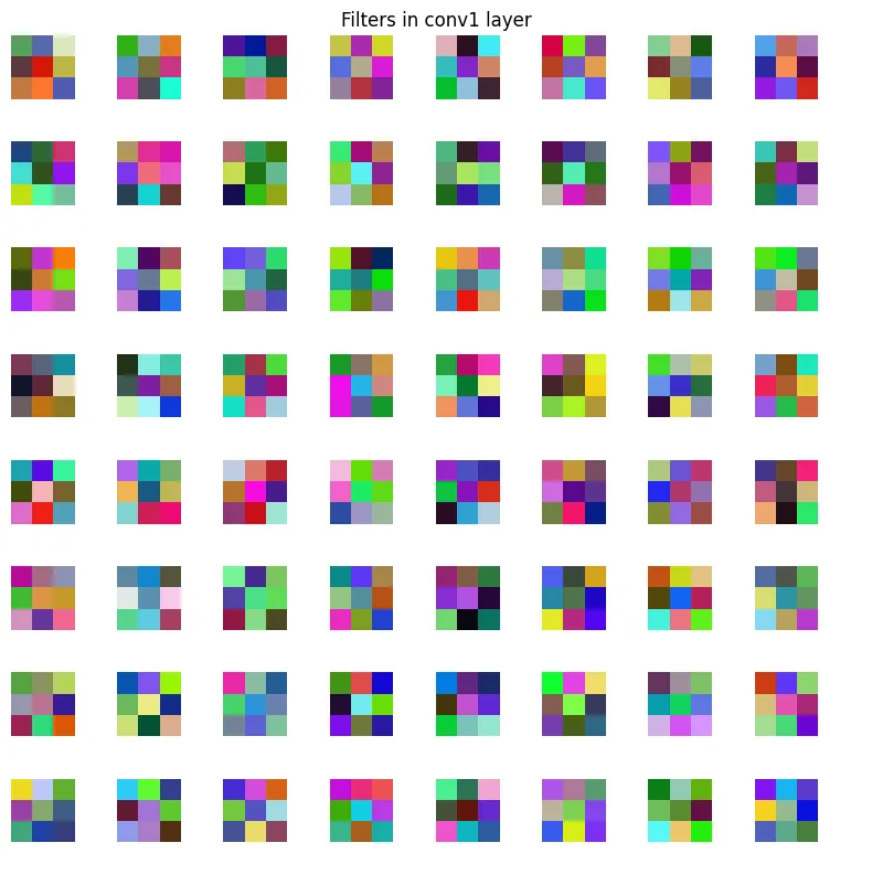
첫번쨰 convolution layer는 RGB형태의 input을 받기 떄문에 첫번쨰 conv1 filter는 RGB image로 변환하여 시각화 할 수 있다. 이후 layer의 filter는 high dimension을 갖기 떄문에 conv layer에 비해 시각화가 어렵다.

해당 layer의 weight를 conv1_filters_data 변수에 할당해서 시각화하기

def plot_filters(data, title=None):
	'''{filter 데이터를 입력으로 받아서 시각화 하는 함수}'''

#VGG11 classification 모델 인스턴스
model = VGG11Classification()
model.load_state_dict(torch.load(model_root))

#모델의 backbone의 attribute conv1의 weight를 data로 불러와서 저장
conv1_filters_data = model.backbone.conv1.weight.data

plot_filters(conv1_filters_data, title="Filters in conv1 layer")

3. Visualizing model activations

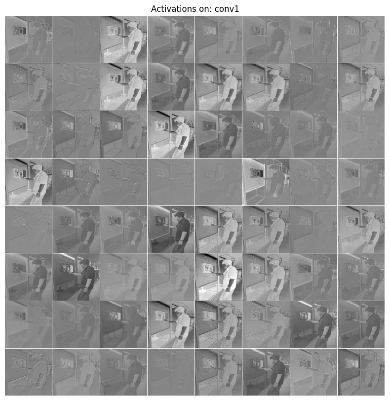
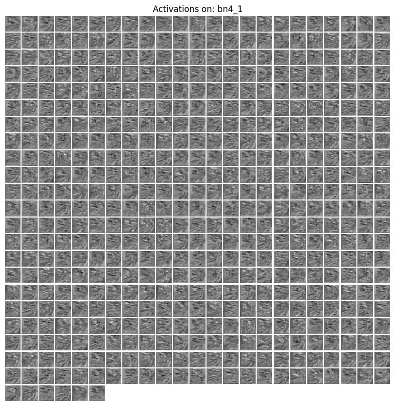
Pytorch에서는 hook을 통해서 최종 출력값이 아닌 중간 layer들의 출력값을 얻을 수 있다. → 모델의 원하는 부분에 hook을 건 다음 해당 layer의 출력을 가져올 수 있다. → 각 layer의 activation을 시각화할 수 있다.

activation_list = []

def show_activations_hook(name, module, input, output):
  # conv/relu layer outputs (BxCxHxW)
  if output.dim() == 4:
    activation_list.append(output)
    plot_activations(output, f"Activations on: {name}")

show_activations_hook 이 함수는 각 layer에 걸어줄 hook함수이다. layer를 거치고 나온 output을 activation list에다가 넣어준 후 이전에 정의해둔 plot_activations() 함수에다가 넣으면 각 layer의 heatmap을 볼 수 있다.

이제 각 module에 forward hook을 걸여줘서 layer의 출력값을 시각화해보자.

module.register_forward_hook사용
functools.partial 을 이용해서 함수의 name 인자가 채워진채로 호출하기 이용

#pretrain된 모델을 불러오고 파라미터를 불러와서 float64로 바꿔줌 -> 이미지와 데이터타입 통일
model = VGG11Classification()
model.load_state_dict(torch.load(model_root))
model.double()

#Hook에 등록할 module담기
module_list  = [model.backbone.conv1, model.backbone.bn4_1]
module_names = ["conv1", "bn4_1"]

#각 module불러와서 register_forward_hook을 이용해서 layer마다 show_activations_hook함수 등록
for idx, (name, module) in enumerate(zip(module_names, module_list)):
  #functools.partial()을 통해서 name인자가 채워진채로 호출
  hook = module.register_forward_hook(functools.partial(show_activations_hook, name))
  module.name = name
  
  #model에 img를 넣어서 hook함수 실행 -> 결과값은 버림
_ = model(img)

conv1 layer와 bn4_1 layer를 거치면서 hook_fn을 거친 결과는 다음과 같다.

Visualizing saliency

saliency map을 시각화해보자.

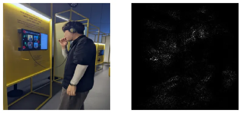
saliency map(중요한 맵):CNN에서 각 pixel이 기여하고 있는 정도를 시각화하여 나타낸 것으로 activation map이라고 불림

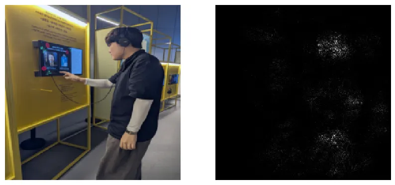
(1) Input image에 대한 gradient s_y(score at index class_idx)를 return하는 함수 compute_gradient_score 만들기

${\partial s_y \over \partial I}$를 계산해서 이미지의 class score($s_y$)에 대한 gradient를 게산할 수 있다.

$s_y$는 class $y$에 대한 logit이다. (softmax layer를 통과하기 이전의 값)

Gradient를 계산한 다음에 해당 값들을 시각화 → input image에 대한 saliency를 확인할 수 있다.

def compute_gradient_score(scores, image, class_idx):
    """
    Returns the gradient of s_y (the score at index class_idx) w.r.t the input image (data), ds_y / dI.

    class_idx에 해당하는 class에 대한 gradient인 s_y를 계산해야 합니다.
    전체 class의 개수의 길이를 갖는 scores에서 원하는 index의 score를 s_y로 얻은 다음, 해당 s_y를 back-propagate하여 gradient를 계산하는 코드를 완성해주세요.
    """
    #grad라는 변수를 image tensor와 동일한 모양의 0으로 채워진 텐서로 초기화
    grad = torch.zeros_like(image)
#목표로 하는 class_idx에 해당하는 스칼라 점수값 선택
    s_y = scores[class_idx]
#s_y에 대한 모든 파라미터 미분
    s_y.backward()
#윗줄에서 계산된 image.grad기울기 텐서값을 grad변수로 가져오기
    grad = image.grad
    assert tuple(grad.shape) == (1, 3, 224, 224)
#계산된 기울기 grad tensor에서 배치차원(인덱스0)을 제거하고 반환
    return grad[0]

계산한 Gradient를 시각화하면 아래사진과 같이 나타난다.

(2) Grad-CAM을 시각화하기

vis_gradcam 함수를 만들자.

Layer의 activation을 저장할 function을 hook하고 forward하기
gradients를 저장하기 위해 hook을 register하고 출력에 대한 최댓값에 해당하는 score를 backwawrd하기

${\partial y^c \over \partial A^k}$를 통해 $\alpha^k_c$를 구할 수 있다.

$y^c$는 class $c$에 대한 score이고, $A^k$는 target layer인 $k$번째 feature map의 Activation이다.

$\alpha^k_c$를 weight로 하여 forwawrd activation maps$A$의 Weighted sum을 얻고, ReLU를 통과하여 $L_{Grad-CAM}^c(i.e,ReLU (\sum_k \alpha_c^k A^k)$를 얻는다.

save_feat=[]
#output feature를 hook_feat에다가 append해서 모아놓기
def hook_feat(module, input, output):
  save_feat.append(output)
  return output

save_grad=[]
#grad를 save_grad 리스트에다가 append해서 모아놓기
def hook_grad(grad):
  """
  중간 layer에서 gradient구하기-> 리스트에 append (dy / dA).
  dy / dA 리턴하기
  """
  save_grad.append(grad)
  return grad

def vis_gradcam(vgg, img):
  """
  gradcam visualization하는 함수
  """
  vgg.eval()

  
  # (1) Reister hook for storing layer activation of the target layer (bn5_2 in backbone)
  # hook_feat의 activation을 register_forward_hook을 이용해서 bn5_2에 등록하기
  vgg.backbone.bn5_2.register_forward_hook(hook_feat)

  # (2) Forward pass to hook features
  # 위에서 hook했으니깐 img forward하기
  img = img.unsqueeze(0)
  s = vgg(img)## FILE ME ##

  # (3) Register hook for storing gradients
  # gradients를 저장하기 위해 hook을 register하기
  save_feat[0].register_hook(hook_grad)

  # (4) Backward score
  # 출력에 대한 최댓값에 해당하는 score를 backward하기
  y = torch.argmax(s)
  s_y = s[0,y]
  s_y.backward()

  # Compute activation at global-average-pooling layer
  # 전역의 average-pooling layer를 통해 activation map 계산
  gap_layer  = torch.nn.AdaptiveAvgPool2d(1)
  alpha = gap_layer(save_grad[1][0].squeeze())
  A = save_feat[0].squeeze()

  # (1) Compute grad_CAM
  # ReLU layer 정의
  # (You may need to use .squeeze() to feed weighted_sum into into relu_layer)
  relu_layer = torch.nn.ReLU()

	# weighted_sum:forward activations maps인 A의 weighted sum구하기
  weighted_sum = torch.sum(save_grad[0].mean(dim=(2,3), keepdim=True) * save_feat[0], dim=1)
  # RelU 통과시키기
  grad_CAM = relu_layer(weighted_sum.squeeze())

  grad_CAM = grad_CAM.unsqueeze(0)
  grad_CAM = grad_CAM.unsqueeze(0)

  # (2) Upscale grad_CAM
  # (You may use defined upscale_layer)
  # grad_CAM 업스케일링 하기
  upscale_layer = torch.nn.Upsample(scale_factor=img.shape[-1]/grad_CAM.shape[-1], mode='bilinear')

  grad_CAM = upscale_layer(grad_CAM)
  grad_CAM = grad_CAM.squeeze()

	#plt 이용해서 grad_CAM시각화하기 
  # Plotting
  #plt 이용하려면 tensor에서 numpy로 바꿔줘야됨
  img_np = image_tensor_to_numpy(img)
  if len(img_np.shape) > 3:
    img_np = img_np[0]
  img_np = normalize(img_np)

  grad_CAM = grad_CAM.squeeze().detach().numpy()

  plt.figure(figsize=(8, 8))
  plt.imshow(img_np)
  plt.imshow(grad_CAM, cmap='jet', alpha = 0.5)
  plt.show

  return grad_CAM

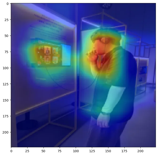— 시각화한 결과 grad_CAM을 시각화해서 Saliency map을 얻어냈다. → 모델의 변형없이 한번의 back_propagation으로 Class activation map을 구함.

Continue exploring

더 읽어보기

모든 글

Project · 2026.10.12