[CV][4주차_과제_1] Vision Transformers
Vision Transformers
과제1_Vision Transformers
문제정의
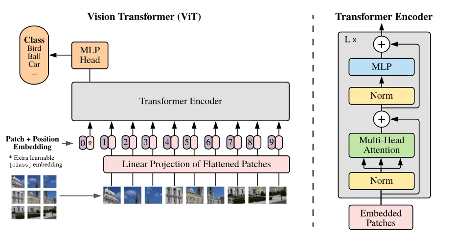
CNN과 달리 ViT는 이미지를 패치로 분할하고, 각 패치를 sequence data로 간주하여 Transformer모델에 입력한다. → CNN에 비해 높은 성능을 발휘한다.
ViT Inference 파이프라인
.png)
- 이미지를 (16*16) stride를 가지는 2D Conv Filter를 이용해서 224*224이미지를 14*14의 패치로 나누기
- Positional Embedding 더하기
- Multi-Head Self-Attention을 통해 Encoding
- MLP Head를 통해 Classification 결과 출력
이미지를 패치로 나누기
Conv2d(3, 768, kernel_size=(16, 16), stride=(16, 16))
Conv2d()를 통해 입력 이미지를 768개의 dimension을 가지는 embedding vector로 변환함
import torch.nn as nn
#이미지를 패치 임베딩으로 변환하는 클래스
class PatchEmbed(nn.Module):
    def __init__(self, img_size=224, patch_size=16, in_chans=3, embed_dim=768):
        super(PatchEmbed, self).__init__()

        # 이미지 사이즈, 패치사이즈, 그리드사이즈, 패치수 정의
        self.img_size = img_size
        self.patch_size = patch_size
        self.grid_size = self.img_size // self.patch_size
        self.num_patches = self.grid_size ** 2

        #Conv2d() 이용해서 임베딩 인스턴스 정의
        self.proj = nn.Conv2d(
            in_channels = 3, #RGB
            out_channels = 768, #임베딩 차원
            kernel_size = 16, # 패치 한개의 크기
            stride = 16 #다음패치로 넘어가려면 16씩 stride
         )


    def forward(self, x):

        #Conv2d()의 인스턴스인 proj()를 통해 임베딩 벡터로 변환하고 flatten, transpose하기
        x = self.proj(x)
        x = x.flatten(2).transpose(1, 2)


        return x
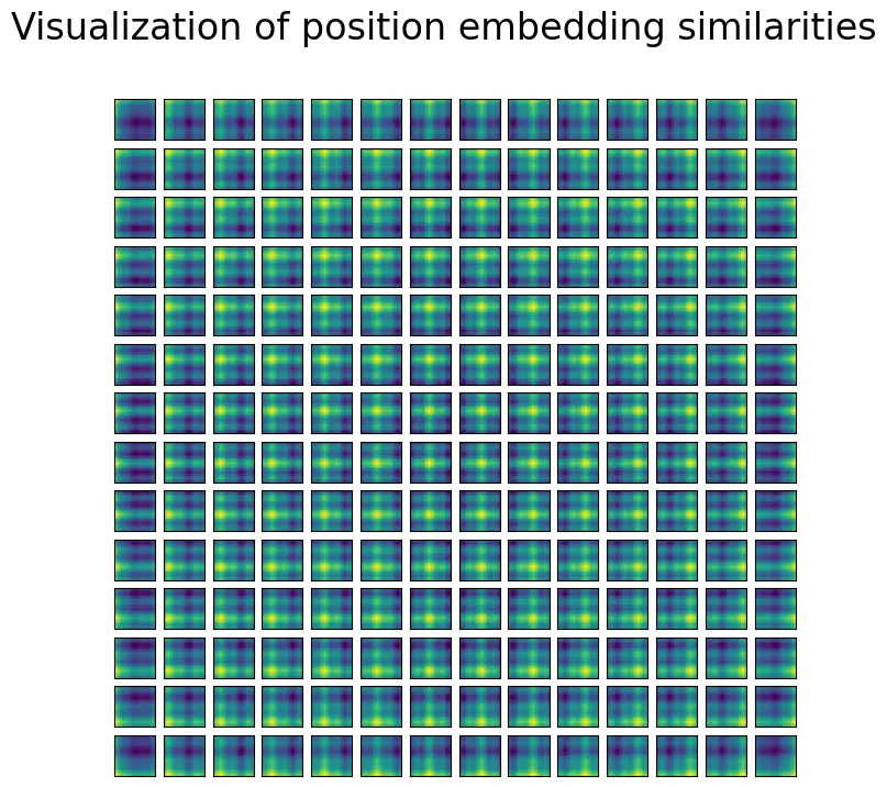
Position Embeddings 더하기
# Position embedding 유사성 시각화
# 하나의 patch와 다른 모든 patch 간의 cosine similarity를 시각화함
cos = torch.nn.CosineSimilarity(dim=1, eps=1e-6)
fig = plt.figure(figsize=(8, 8))
fig.suptitle("Visualization of position embedding similarities", fontsize=24)
for i in range(1, pos_embed.shape[1]):

  ## 현재 패치의 임베딩과 모든 패치의 임베딩 사이에 코사인 유사도 구하기
    sim = F.cosine_similarity(pos_embed[0,i:i+1],pos_embed[0,1:])#.detach().cpu().numpy()
    #유사도 벡터 sim을 패치 그리드 형태로 재배열
    sim = sim.reshape((14,14))
    #plt를 이용하기 위해 detach한 후 cpu에다 올리기
    sim = sim.detach().cpu().numpy()

    #시각화
    ax = fig.add_subplot(14, 14, i)
    ax.axes.get_xaxis().set_visible(False)
    ax.axes.get_yaxis().set_visible(False)
    ax.imshow(sim)
Transformer Input 생성
학습가능한 class token이 patch embedding vector의 1번째 순서에 합쳐져야 한다. 각 패치들의 Attention결과 값은 버려지고 Class token의 결과값만 MLP Head에 들어간다.
transformer_input = torch.cat((model.cls_token, patches), dim = 1) + pos_embed
기존의 패치와 cls_token 을 concat한 후, pos_embed 을 더한다.
Transformer Encoder
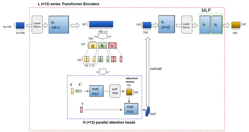
- N = 197(cls_token + patches) embedded vector가 들어감
- qkv에 Multihead attention을 적용하기 위해 12(H)개로 분리
- Attention연산을 거친 후 output을 concat한 후 fc layer통과
# Multi-head attantion을 위해 qkv를 여러개의 q, k, v vector들로 나누기
qkv = transformer_input_expanded.reshape(197, 3, 12, 64)  # (N=197, (qkv), H=12, D/H=64)
print("split qkv : ", qkv.shape)
q = qkv[:, 0].permute(1, 0, 2)  # (H=12, N=197, D/H=64)
k = qkv[:, 1].permute(1, 0, 2)  # (H=12, N=197, D/H=64)
kT = k.permute(0, 2, 1)  # (H=12, D/H=64, N=197)
print("transposed ks: ", kT.shape)
# Attention Matrix
atten = torch.matmul(q,kT)/8.0
attention_matrix = F.softmax(atten, dim = -1)
#attention_matrix = torch.matmul(atten, qkv[:,2].permute(1,0,2))
print("attention matrix: ", attention_matrix.shape)
plt.imshow(attention_matrix[3].detach().cpu().numpy()
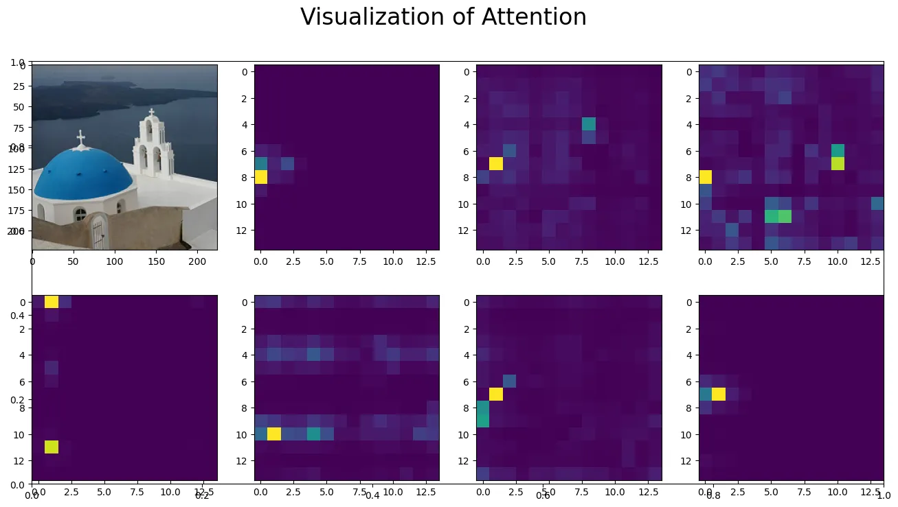
softmax() 연산을 거친 attention_matrix를 계산한 후 시각화한다.
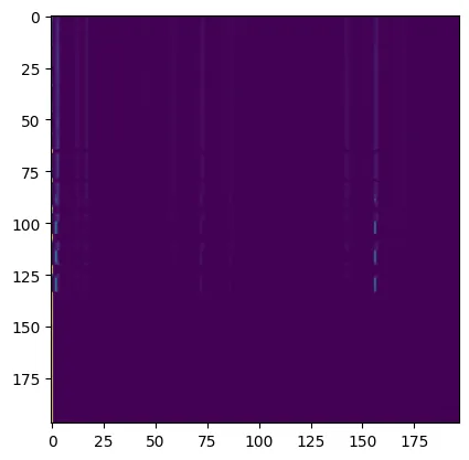
각 0~7까지의 Multi head Attention에서 Attend하는부분을 시각화해서 확인하기
# Attention matrix 시각화
fig = plt.figure(figsize=(16, 8))
fig.suptitle("Visualization of Attention", fontsize=24)
fig.add_subplot()
img = np.asarray(img)
ax = fig.add_subplot(2, 4, 1)
ax.imshow(img)
for i in range(7):  # 0-7번째 헤드들의 100번째 줄(row)의 attention matrix 시각화
    attn_heatmap = attention_matrix[i, 100, 1:].reshape((14, 14)).detach().cpu().numpy()
    ax = fig.add_subplot(2, 4, i+2)
    ax.imshow(attn_heatmap)
MLP Head
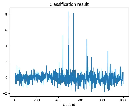
Multi-Head Self-Attention을 거친 후 가장 확률이 높은 클래스를 MLP Head에서 예측해낸다.
Continue exploring
더 읽어보기
CTR을 예측할 수 있을리가 없잖아 무리무리!(무리가아니었다!?): nemotron persona
어떤 광고 배너가 잘될지는 결국 집행 비용을 써봐야 알 수 있었다. 배너를 많이 만들 수 있어도, 그중 무엇을 내보낼지 고르는 데는 여전히 돈이 들었다. 집행 전에 후보를 걸러낼 수 있을지 확인하려고 NVIDIA Nemotron Persona-Korea 데이터셋으...
카피 A/B 테스트와 밈으로 광고 성과를 끌어올리기
광고 배너를 자동으로 만들 수 있게 된 뒤에는 어떤 카피를 얹을지가 다음 과제였다. 성과가 높은 카피, 재밌는 카피에는 정해진 Ground Truth가 없었다. 여러 톤앤매너와 밈 RAG로 후보를 만들고 실제 광고 성과를 비교했다.
성과가 난 광고에서 다음 스토리를 찾는 위닝앵글 검색
초기 AX 제작은 좋아요 랭킹 순으로 스토리를 넓게 탐색하는 방식이었다. 이후에는 이미 성과가 난 광고에서 다음 후보를 찾는 경로를 만들었다. 다른 팀원이 만든 에이전트의 광고 성과 분석과 인사이트를 받아, 비슷한 소구점이나 이미지를 가진 새로운 스토리를 발굴하는...