Study

[PyTorch][1주차_기본과제_1] Tensor의 생성/조작/연산

Tensor의 생성/조작/연산

Published 2025.10.06 Reading 7 minute read

과제1_Tensor의 생성/조작/연산

Pytorch를 이용한 Tensor의 생성/조작/연산에 익숙해지기

Task 1. Tensor의 자료형 조작
Task 2. Tensor의 생성
Task 3. CUDA Tensor와 연산
Task 4. Tensor의 모양 변경
Task 5. 유사도
Task 6. Tensor를 활용한 이미지의 이해(응용)
Task 7. Tensor를 조작하여 이미지 data augmentation 하기(응용)

Tensor의 Data Type 조작

#10.2의 값을 64-bit floating point인 1-D Tensor 't'를 정의
t = torch.tensor(10.2, dtype=torch.float64)
print("t: {}".format(t))

#t Tensor의 자료형을 출력하기.
print(t.dtype)

# t Tensor의 자료형을 32-bit integer (signed)로 변환.
t = t.int()

# t Tensor의 자료형을 32-bit floating point (signed)로 변환
t = t.float()

tensor.dtpye : data type을 반환한다.

torch.tensor() 괄호 안에 있는 리스트나, 스칼라값을 tensor로 만든다. 이때 dtype을 따로 정의해줄 수 있다.

torch.int() : singed 32bit integer로 torch의 data type 바꿔주기

torch.float(): tensor의 datatype을 32bit float으로 바꾸기

자료형 변환 후(float → int → float) tensor의 값이 같을까?

float을 int로 변환 후 다시 float으로 변환시키면 소숫점 아래를 버려서 값이 달라지게 된다.

Tensor의 생성

#초기화 되지 않은, [2,4] shape의 tensor를 생성
empty_t = torch.empty(2,4)

#empty_t Tensor가 메모리 상에서 고유한 식별자 출력
print(id(empty_t))
print('\n')

# empty_t의 요소들에 1로 값을 채워주세요.
ones_t = torch.ones_like(empty_t)
print('ones_t: {}'.format(ones_t))

# ones_t Tensor가 메모리 고유한 식별자를 출력
print(id(ones_t))
print('\n')

#empty_t 의 요소들에 0으로 값 채우기. 단, in-place 방식을 이용
zeros_t = empty_t.zero_()
print('zeros_t: {}'.format(zeros_t))

#zeros_t Tensor가 메모리상 고유한 식별자 출력
print(id(zeros_t)

torch.empty(shape) 초기화 되지 않은 상태로 shape을 지정해서 tensor를 생성

id(torch) : torch의 메모라상의 id를 반환함

zeros_t의 id와 empty_t의 id가 같고 값이 동일한가?

empty_t에서 inplace방식으로 0을 채워줬기 때문에 id가 같아야 한다.

하지만 ones_t는 ones_like 로 생성했기 때문에 id가 다르다.
torch.fill_은 초기화 되지 않은 tensor에 다른 데이터로 수정하는 표현이다. → 메모리주소는 그대로고 값만 변경된다.

# 크기가 30인 표준정규분포 난수 Tensor를 생성
rand_t =  torch.randn(30)

#rand_t의 shape 을 출력
print(rand_t.shape)

#rand_t가 0차원은 1, 1차원은 3을 가지도록 shape을 변경
v_t = rand_t.view(1,3,-1)
print("v_t.shape: {}".format(v_t.shape))

# v_t 와 shape이 같으면서 1으로 채워진 Tensor를 생성
ones_t = torch.ones_like(v_t)

torch.randn(shape) : shape사이즈만큼의 표준 정규분포 난수 Tensor를 생성

torch.view(1,3,-1) depth는 1차원, 행은 3차원, 열은 10차원을 갖도록 변경

view는 메모리구조상 contigious할때만 사용할 수 있으므로, 슬라이싱한 텐서에서는 사용할 수 없음.

CUDA Tensor와 연산

# CUDA가 사용가능한지 출력
print(torch.cuda.is_available())
# 사용가능한 GPU 개수를 출력
print(torch.cuda.device_count)
#CUDA device이름 출력
print(torch.cuda.get_device_name(device = 0))
# TODO 3-4) CUDA가 사용 가능하면 'cuda'를, 그렇지 않으면 'cpu'를 device라는 변수명에 대입
device = 'cuda' if torch.cuda.is_available() else 'cpu

#arange()이용해서 tensor 생성하기
tensor_1 = torch.arange(0,1000,0.001)

tensor_2 = torch.arange(0,10000,0.01)

‘GPU’라는 장치는 없고 ‘cuda’ 아니면 ‘cpu’ 중 하나에 올려서 tensor를 사용해야됨

numpy나 matplotlib을 사용할때는 to(’cpu’) 를 이용해서 tensor를 cpu에 올려서 사용하고, 학습이나 추론을 할때는 to(’cuda’) 를 이용해서 tensor를 GPU에 올려서 사용해야됨

arange는 array range 의 줄임말이라서 arrange로 잘못사용하는것 주의하기

torch.arange() :시작범위와 끝범위 stepping을 정의해서 해당 범위의 값을 갖는 tensor를 생성함

def tensor_operations(t1, t2, prt=True):
  ot1 = t1.clone()
  ot2 = t2.clone()
  # 시간측정
  start_time = time.time()

  # in-place 방식을 활용하여 t1에 t2를 더하기
  t1.add_(t2)
  # t1에서 t2를 뺀 후 t3에 대입
  t3 = torch.sub(t1,t2)
  #in-place 방식을 활용하여 t3에 1.2를 곱하기
  t3.mul_(1.2)

  # t3에서 2를 나눈 후 t4에 대입
  t4 = torch.div(t3, 2)
  # in-place 방식으로 t4를 제곱.
  t4.pow_(2)

  end_time = time.time()

연산에서 inplace방식을 사용하고싶으면 add, mul, div, sub 뒤에 언더스코어(_)를 붙여서 사용하기

두 tensor를 gpu에 올리기

tensor_c1 = torch.tensor(tensor_1).to('cuda')
tensor_c2 = torch.tensor(tensor_2).cuda()

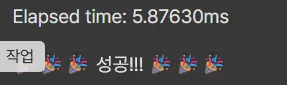
tensor가 cpu에 있을때의 연산 시간

tensor를 gpu에 올리고 나서 연산시간

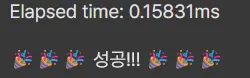
cpu보다 gpu에 올리고 나서 연산이 매우 빨라진 것을 알 수 있다.

Tensor의 Shape 변경

# 0부터 10까지 1씩 증가하는 1-D Tensor를 생성
t = torch.arange(0,10,1)
print("t.shape: {}".format(t.shape))

# t Tensor의 shape을 [2, 5]로 변경
reshaped_t = t.reshape(2,5)
# reshaped_t Tensor의 shape을 확인하여 출력
print(t.shape)
# t Tensor의 shape 을 [2, 5]로 변경
v_t = t.view(2,5)
# v_t Tensor의 shape을 확인하여 출력
print(v_t.shape)

# v_t Tensor의 contiguous 속성을 확인

print(v_t.is_contiguous())
# v_t Tensor에서 0차원은 전부, 1차원은 0번째 요소부터 3번째까지 slicing
sliced_t = v_t[:,:4]
#sliced_t Tensor의 contiguous 속성을 확인
print(sliced_t.is_contiguous()

tensor.reshape() :view() 와 다르게 contigious하지 않아도 텐서의 모양을 변경할 수 있지만, inplace방식이 아니라 복사해서 출력하는것이므로 메모리사용량이 많음

tensor.is_contigious() :텐서가 메모리상에서 contigious한지 boolean값으로 반환 → 슬라이싱 한 후의 Tensor는 contigious하지 않음

다만 tensor.contigious 속성을 사용하면 tensor를 contigious하게 바꿔줄 수 있음

# 0번째 차원은 1, 1번째 차원은 2, 2번째 차원은 2, 3번째 차원은 1,
# 4번째 차원은 나머지를 가지도록 sliced_t의 shape을 변경.

reshaped_t = sliced_t.reshape(1,2,2,1,-1)
print("reshaped_t.shape: {}\n".format(reshaped_t.shape))

# reshaped_t Tensor의 2번째 차원부터 마지막 차원까지 평탄화
flatten_t = torch.flatten(reshaped_t,2)
print("flatten_t.shape: {}".format(flatten_t.shape))
print("flatten_t : {}".format(flatten_t)

torch.flatten(tensor,idx) : tensor의 idx차원부터 마지막 차원까지 평탄화 하기

# 0부터 12까지 1씩 증가하는 1-D Tensor를 생성
t = torch.arange(0,12,1)
print("t: {}".format(t))

# t Tensor의 shape을 [2, 2, 3]으로 변경
t = t.reshape(2,2,3)
print("t: {}\n".format(t))

# t Tensor의 2번째 차원과 1번째 차원을 바꾸기
transposed_t = t.transpose(2,1)
print("transposed_t: \n{}".format(transposed_t))
print("transposed_t.shape: {}\n".format(transposed_t.shape))

# 차원의 축을 변경하지 않고 t Tensor의 shape 을 [2, 3, 나머지]로 변경
reshaped_t = t.reshape(2,3,-1)
print("reshaped_t: \n{}".format(reshaped_t))
print("reshaped_t.shape: {}\n".format(reshaped_t.shape)

tensor.transpose(idx_1,idx_2) : idx_1차원과 idx_2차원을 바꾸기

Transpose를 적용한 transposed_t 와 reshape을 적용한 reshaped_t 는 같을까?

결과는 다르고 모양은 [2,3,2]로 같다. transpose는 reshape과 달리 Tensor의 특정한 두 차원의 축을 서로 바꾸는 메서드이기 때문이다.

# t Tensor에서 0차원으로 dim이 1인 차원 확장.
t = t.unsqueeze(0)
print("t.shape: {}".format(t.shape))

# t Tensor에서 2차원으로 dim이 1인 차원 확장.
t = t.unsqueeze(2)  
print("t.shape: {}".format(t.shape))

# t Tensor에서 마지막 차원으로 dim이 1인 차원 확장
t = t.unsqueeze(-1) 
print("t.shape: {}".format(t.shape)

유사도

맨해튼 유사도

# 맨해튼 유사도를 구하는 함수를 정의
def get_manhattan_similarity(t1, t2):
	#맨해튼 거리는 L1 norm상에서의 거리
  manhattan_distance = torch.norm(t1-t2, p=1)
	#맨해튼 유사도 공식적용
  manhattan_similarity = 1/(1+manhattan_distance)
  print("manhattan_similarity: {}".format(manhattan_similarity))
	# 맨해튼 유사도 return
  return manhattan_similarity 

유클리드 유사도

# 유클리드 유사도를 구하는 함수를 정의
def get_euclidean_similarity(t1, t2):
	# 유클리드 거리는 L2 norm 상에서의 거리
  euclidean_distance = torch.norm(t1-t2, p=2)
	#유클리드 유사도 공식 적용
  euclidean_similarity = 1/(1+euclidean_distance)
  print("euclidean_similarity: {}".format(euclidean_similarity))
  return euclidean_similarity 

코사인 유사도

# 코사인 유사도를 구하는 함수를 정의
def get_cosine_similarity(t1, t2):
	#코사인유사도 공식 적용 -> L2 norm 사용
  cosine_similarity = torch.dot(t1,t2)/(torch.norm(t1,p=2)*torch.norm(t2,p=2))
  print("cosine_similarity: {}".format(cosine_similarity))
  return cosine_similarity

t1 = torch.tensor([1., 2., 0., 3., 5.])
t2 = torch.tensor([2., 1., 1., 1., 0.])

manhattan_s = get_manhattan_similarity(t1,t2)

euclidean_s = get_euclidean_similarity(t1,t2)

cosine_s = get_cosine_similarity(t1,t2)

t1, t2텐서의 코사인, 유클리디안, 맨해튼 유사도를 구하기

Tensor를 활용한 이미지의 이해

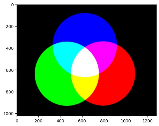
컬러이미지는 red, green, blue 세개의 채널로 이루어져 있따. 세개의 채널이 조합되어 하나의 컬러 이미지를 출력한다. 반면 흑백 이미지는 하나의 채널만을 가진다.

# numpy array인 image로 부터 Tensor를 생성
img_t = torch.tensor(image)
# img_t의 data type을 출력
print(img_t.dtype)
>>> torch.uint8

이미지는 크기만큼 (Height*width)픽셀이 존재하며 하나의 픽셀은 (R,G,B) 세개의 채널을 갖는다. → 이미지는 3차원…

Tensor조작하여 data augmentation하기

def add_random_noise(img_t, scale=30):
  # img_t와 모양(shape)이 같은 표준정규분포 난수 Tensor를 생성
  random_noise = torch.randn_like(img_t.float())
  print("random_noise.mean: {:.4f}".format(random_noise.mean()))
  print("random_noise.std: {:.4f}".format(random_noise.std()))
  print("random_noise.min: {:.4f}".format(random_noise.min()))
  print("random_noise.max: {:.4f}\n".format(random_noise.max()))

  random_noise *= scale

  # img_t의 자료형을 32-bit floating point로 변환한 후 random_noise를 더해 주기
 
  img_t = img_t.float()
  noise_added_img = torch.add(img_t,random_noise)
  # noise_added_img의 모든 값이 0과 255 사이의 값을 가지도록 제한 - cliping
  noise_added_img = noise_added_img.clip(0,255)
  # noise_added_img의 자료형을 torch.uint8로 변환
	noise_added_img =noise_added_img.type(torch.uint8)

  print("noise_added_img.min: {}".format(noise_added_img.min()))
  print("noise_added_img.max: {}\n".format(noise_added_img.max())

노이즈가 들어가기전 이미지

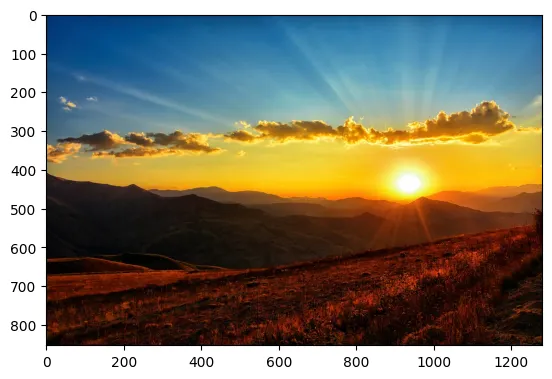
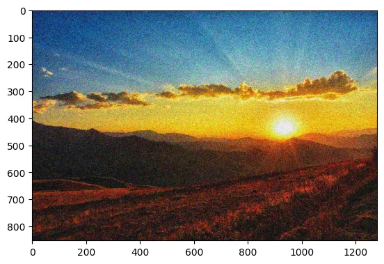
노이즈가 들어간 후 이미지

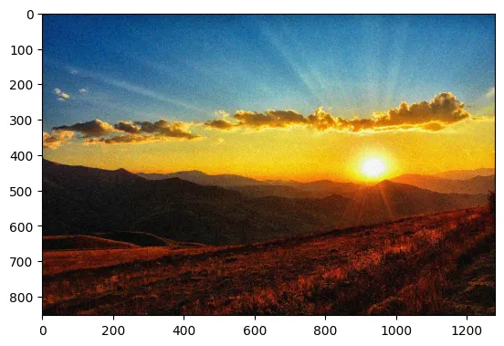
plt.imshow(add_random_noise(img_t, scale=55)

노이즈의 scale을 조정하면서 노이즈의 변화에 따른 이미지를 시각화 할 수 있다. → noise의 값이 과하지 않도록 값을 제한하는 것이 좋다. 이미지는 uint8 로 0~255사이의 값을 가짐을 고려.

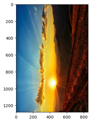
img_tp = img_t.transpose(0,1)

0차원과 1차원을 transpose해줌으로써 가로세로 방향을 바꿀 수도 있다.

Continue exploring

더 읽어보기

모든 글

Project · 2026.10.12