[RecSys][과제3] 추천시스템을 위한 생성모델 구현
[RecSys][과제3] 추천시스템을 위한 생성모델 구현
과제3_추천시스템을 위한 생성모델 구현
- AutoEncoder기반 추천시스템 모델(AutoRec)을 학습시킨다.
- 생성모델 기반 추천시스템 모델을 학습시킨다.
- 추천시스템에서 생성모델이 어떻게 활용되는지 자세히 알아보자.
- Autoencoder를 활용한 추천시스템 모델인 AutoRec에 대해서도 배운다.
- Variational Inference 기반의 variational autoencoder(VAE)를 직접 학습시켜보며, 이를 추천시스템에 적용해 보자.
데이터셋
과제 2와 마찬가지로 MovieLens Dataset을 사용한다.
출처 :Harper, F. M., & Konstan, J. A. (2015). The MovieLens Datasets: History and Context.
ACM Transactions on Interactive Intelligent Systems (TIIS), 5(4), 1-19. http://dx.doi.org/10.1145/2827872
과제 2와 마찬가지로 평점 데이터는 ratings_df 로 불러오고, 영화 정보 데이터는 movies_df 로 불러온다.
df_train, df_test = train_test_split(
    user_item_matrix, test_size=0.2, random_state=42)
그리고 df_train과 df_test로 train_test_split() 을 이용해서 train_dataset과 test_dataset으로 나눠준다.
AutoRec 모델 구현하기
2015년에 제안된 모델로 추천시스템 설계시, 사용자와 항목을 복합적으로 고려하는 “Collaborative filtering”을 위해 설계된 모델이다.
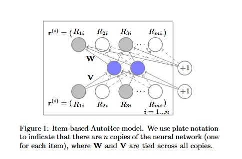
\(r^{(i)}$는 각각의 n개의 item에 대한 rating을 담고있는 input이자 output이다. input으로\)r^{(i)}$$를 넣어주면 모델을 거쳐서 masking된(빈칸) 입력에 대한 output rating을 예측(reconstruction)하는 모델이다.
class AutoRec(nn.Module):
    def __init__(self, input_size, hidden_size):
        super(AutoRec, self).__init__()
        self.encoder = nn.Linear(input_size, hidden_size)
        self.decoder = nn.Linear(hidden_size, input_size)

    def forward(self, ratings):
        encoded = torch.sigmoid(self.encoder(ratings))
        decoded = self.decoder(encoded)
        return decoded
AutoRec 클래스를 통해 모델을 구현한다. 구조 자체는 간단한데, 선형변환 nn.Linear() 로 encoding 과 decoding layer를 정의한다. 그리고 forward() 에서는 들어온 ratings를 encode() 하고 Activation Function에 넣어준 후 다시 decode() 해준다.
# 하이퍼파라미터 설정
hidden_size = 10
learning_rate = 0.001
num_epochs = 20
lambda_value = 0.001  # weight decay의 계수

# 데이터 로더 생성
train_dataset = TensorDataset(torch.Tensor(df_train.values))
train_loader = DataLoader(train_dataset, batch_size=64, shuffle=True)

num_movies = user_item_matrix.shape[1]

# 모델 초기화
model = AutoRec(num_movies, hidden_size)
criterion = nn.MSELoss(reduction="sum")
optimizer = optim.Adam(model.parameters(), lr=learning_rate)
하이퍼파라미터로 epoch수와, weight_decay의 계수, lr, hidden_size를 설정한다.
데이터로더로 train_dataset을 불러오고, 만든 모델을 불러오고, MSELoss() 로 lossfunction을 사용하고, Adam() 으로 Optimizer를 불러온다..
AutoRec 학습과정 구현하기
#model parameter에 L2-regulation항을 더해준다.->Overfitting을 막기 위함
def weight_decay_loss(model, lambda_value):
    l2_reg = None
    for param in model.parameters():
        if l2_reg is None:
            l2_reg = param.norm(2)
        else:
            l2_reg = l2_reg + param.norm(2)
    return lambda_value * l2_reg

#true_positive/sum(y_true)을 계산해서 k에서의 recall을 계산한다.
def recall_at_k(y_true, y_score, k):
    """Compute Recall@k"""
    _, indices = torch.topk(y_score, k, dim=1)
    recalls = []
    for i in range(len(y_true)):
        true_positives = torch.sum(y_true[i][indices[i]])
        recall = true_positives / torch.sum(y_true[i])
        recalls.append(recall.item())
    return torch.tensor(recalls).mean()

# 모델 학습
for epoch in range(num_epochs):
    running_loss = 0.0
    for data in train_loader:
        inputs = data[0]
        optimizer.zero_grad()
        outputs = model(inputs)
        # loss를 정의할떄 앞서 정의한 weight_decay_loss()함수를 통해 L2-reg term을 더해준다.
        loss = criterion(inputs,outputs) + 0.5*weight_decay_loss(model, lambda_value)
        loss.backward()
        optimizer.step()
        running_loss += loss.item()
    running_loss = running_loss/len(train_loader)

    with torch.no_grad():
        test_batch_data = torch.Tensor(df_test.values)
        test_recon_batch = model(test_batch_data)
        test_loss = criterion(test_recon_batch * torch.sign(test_batch_data), test_batch_data).item()

        test_recon_batch_prob = torch.sigmoid(test_recon_batch)

        # NDCG@k와 Recall@k 계산
        ndcg = ndcg_score(df_test.values, test_recon_batch_prob, k=20)
        recall = recall_at_k(test_batch_data, test_recon_batch_prob, k=20)
        mse = mean_squared_error(df_test.values, test_recon_batch * torch.sign(test_batch_data))

        print('Epoch [{}/{}]'.format(epoch+1, num_epochs))
        print('Train Loss: {:.4f}, Test Loss: {:.4f}, NDCG@k: {:.4f}, Recall@k: {:.4f}, MSE: {:.4f}'.format(running_loss, test_loss, ndcg, recall, mse))
Epoch [1/20]
Train Loss: 98700.3874, Test Loss: 268948.0625, NDCG@k: 0.0971, Recall@k: 0.0155, MSE: 0.8460
Epoch [2/20]
Train Loss: 95074.2370, Test Loss: 267445.3125, NDCG@k: 0.1482, Recall@k: 0.0288, MSE: 0.8413
Epoch [3/20]
Train Loss: 94061.6576, Test Loss: 266039.7188, NDCG@k: 0.1760, Recall@k: 0.0408, MSE: 0.8369
Epoch [4/20]
Train Loss: 93309.4954, Test Loss: 264639.8750, NDCG@k: 0.1938, Recall@k: 0.0470, MSE: 0.8325
Epoch [5/20]
Train Loss: 92635.5046, Test Loss: 263226.9375, NDCG@k: 0.2044, Recall@k: 0.0523, MSE: 0.8280
Epoch [6/20]
Train Loss: 91997.1159, Test Loss: 261829.7812, NDCG@k: 0.2128, Recall@k: 0.0564, MSE: 0.8236
Epoch [7/20]
Train Loss: 91397.5404, Test Loss: 260383.3750, NDCG@k: 0.2223, Recall@k: 0.0604, MSE: 0.8191
Epoch [8/20]
Train Loss: 90798.6120, Test Loss: 258914.1875, NDCG@k: 0.2325, Recall@k: 0.0658, MSE: 0.8145
Epoch [9/20]
Train Loss: 90196.8542, Test Loss: 257142.3281, NDCG@k: 0.2388, Recall@k: 0.0694, MSE: 0.8089
Epoch [10/20]
Train Loss: 89436.3372, Test Loss: 253187.0000, NDCG@k: 0.2401, Recall@k: 0.0768, MSE: 0.7964
Epoch [11/20]
Train Loss: 88285.2878, Test Loss: 248248.8594, NDCG@k: 0.2474, Recall@k: 0.0835, MSE: 0.7809
Epoch [12/20]
Train Loss: 86599.3307, Test Loss: 239259.5469, NDCG@k: 0.2546, Recall@k: 0.0915, MSE: 0.7526
Epoch [13/20]
Train Loss: 84050.0820, Test Loss: 228116.2500, NDCG@k: 0.2736, Recall@k: 0.1020, MSE: 0.7176
Epoch [14/20]
Train Loss: 80977.6885, Test Loss: 216019.7188, NDCG@k: 0.2822, Recall@k: 0.1038, MSE: 0.6795
Epoch [15/20]
Train Loss: 78176.8203, Test Loss: 206886.3750, NDCG@k: 0.2947, Recall@k: 0.1049, MSE: 0.6508
Epoch [16/20]
Train Loss: 76111.8548, Test Loss: 199785.7031, NDCG@k: 0.3138, Recall@k: 0.1122, MSE: 0.6285
Epoch [17/20]
Train Loss: 74581.3831, Test Loss: 194842.3594, NDCG@k: 0.3329, Recall@k: 0.1202, MSE: 0.6129
Epoch [18/20]
Train Loss: 73391.6566, Test Loss: 190565.3438, NDCG@k: 0.3520, Recall@k: 0.1294, MSE: 0.5995
Epoch [19/20]
Train Loss: 72376.0072, Test Loss: 187072.0469, NDCG@k: 0.3683, Recall@k: 0.1407, MSE: 0.5885
Epoch [20/20]
Train Loss: 71430.9642, Test Loss: 183538.0312, NDCG@k: 0.3844, Recall@k: 0.1477, MSE: 0.5773
Epoch마다 출력되는 값을 보면 Train Loss와 test Loss모두 줄어드는 경향성을 볼 수 있고, MSE도 줄어드는 경향성을 볼 수 있다.
VAE 모델 구현하기
VAE는 encoder-decoder구조를 사용하는 generative model롷 입력 데이터를 압 축한 후 다시 복원하는 과정을 통해 데이터를 생성한다. VAE는 잠재 변수 공간을 학습하여, 데이터의 Hidden feature를 포착하고, 새로운 데이터를 생성한다.
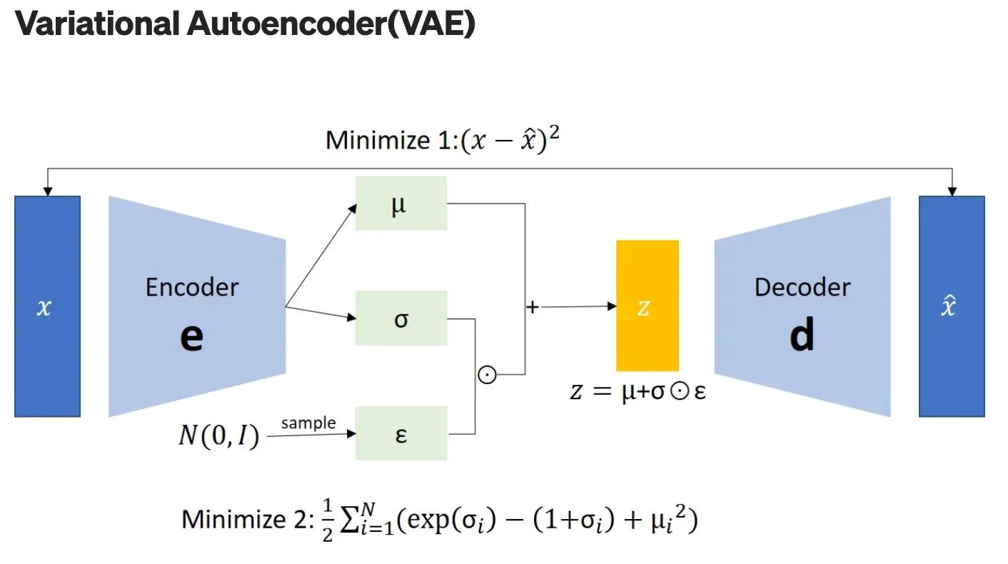
Gaussian distribution을 따르는 \(N(0,1)\) 에서 \(\epsilon\)을 sampling한다.
train을 통해서 z를 학습시킨다. 만약 z가 gaussian N(0,1)을 따른다고 가정할때 x를 출력시켜보면, 원하는 결과를 얻지 못한다. 왜냐하면 데이터에 따른 z가 학습된것이 아니라 임의의 학률분포를 가정한것이기 때문이다.
이때 p(z)는 N(0,1) gaussian 분포를 따르도록 임의로 initializing하고 z와 KL-divergence가 가까워지도록 학습시킨다.
그러면 z와 p(z)가 KL-divergence가 가깝게 만들어줄 수 있다. 하지만 KL-divergence는 확률분포사이의 거리이기 때문에 z를 그대로 써줄 수 없다.
\[KL(q(z\mid x)\mid \mid p(z))\]따라서 x가 주어졌을때 z의 확률분포로 식을 바꿔준 후 KL divegence를 계산한다.
class VAE(nn.Module):
    def __init__(self, input_dim, latent_dim, lambda_value=0.001):
        super(VAE, self).__init__()
        self.input_dim = input_dim
        self.latent_dim = latent_dim
        self.lambda_value = lambda_value

        # 인코더 정의
        self.encoder = nn.Sequential(
            nn.Linear(input_dim, 512),
            nn.ReLU(),
            nn.Linear(512, 256),
            nn.ReLU(),
            nn.Linear(256, latent_dim * 2) #mu, logvar을 동시에 출력
        )

        # 디코더 정의
        self.decoder = nn.Sequential(
            nn.Linear(latent_dim, 256),
            nn.ReLU(),
            nn.Linear(256, 512),
            nn.ReLU(),
            nn.Linear(512, input_dim),
        )
	#mu, logvar, eps를 이용해서 z를 출력한다.
    def reparameterize(self, mu, logvar):
        std = torch.exp(0.5 * logvar)
        eps = torch.randn_like(std)
        return mu + eps * std

    def forward(self, x)
        encoded = self.encoder(x)
        #encoded에 있는 mu와 logvar를 리스트 슬라이싱으로 가져온다.
        mu, logvar = encoded[:,:self.latent_dim], encoded[:,self.latent_dim:]
        #z를 reparameterize함수를 이용해서 계산한다.
        z = self.reparameterize(mu, logvar)
        decoded = self.decoder(z)
				#decoded된 output과 mu, logvar를 출력한다.
        return decoded, mu, logvar
- 인코더: 입력 데이터를 encoding해서 잠재변수의
mu, logvar를 출력한다. reparameterize(): mu, logvar를 이용해서 잠재변수 z를 샘플링한다.- decoder: 잠재변수 z를 decoding해서 원래 입력 데이터의 복원된 값을 출력한다
VAE 손실함수 정의
VAE모델에서 Minimize해야할 목적식은 2개가 있다.
\({MSE} =\sum_{i=1}^{N} \mid x_i - \hat{x}_i\mid ^2_2\) 를 이용해서 입력데이터와 decoder를 거쳐 나온 출력간의 차이를 최소화한다.
\({KLD} = -\frac{1}{2} \sum_{i=1}^{D} (1 + \log(\text{var}) - \mu^2 - \exp(\log(\text{var})))\)를 이용해서 잠재변수의 확률분포$N(\mu,\Sigma)$와 표준 Gaussian distribution $p(z)$ 간의 KL-divergence를 최소화 한다. 이를통해 잠재공간을 구조화 해서 Gaussian distribution과 가깝게 만들어주는 정규화를 하는 것이다.
\(D_{KL}(q_{\phi}(z\mid x)\mid\mid p(z))\)를 minimize하는것과 같다.
# 손실 함수 정의
def loss_function(recon_x, x, mu, logvar):
    MSE = nn.functional.mse_loss(recon_x,x)    ## FILL HERE ##
    KLD = -0.5*torch.sum(1+logvar - mu**2-torch.exp(logvar))
    return MSE + KLD
VAE 모델학습
# 모델 학습
for epoch in range(num_epochs):
    running_loss = 0.0
    for data in train_loader:
        inputs = data[0]
        optimizer.zero_grad()
        outputs, mu, logvar = model_vae(inputs)
        loss = loss_function(outputs, inputs, mu, logvar)
        loss.backward()
        optimizer.step()
        running_loss += loss.item()
    running_loss = running_loss/len(train_loader)

    with torch.no_grad():
        test_batch_data = torch.Tensor(df_test.values)
        test_recon_batch, test_mu, test_logvar = model_vae(test_batch_data)
        test_loss = loss_function(test_recon_batch, test_batch_data, test_mu, test_logvar).item()

        test_recon_batch_prob = torch.sigmoid(test_recon_batch)

        # NDCG@k와 Recall@k 계산
        ndcg = ndcg_score(df_test.values, test_recon_batch_prob, k=20)
        recall = recall_at_k(test_batch_data, test_recon_batch_prob, k=20)
        mse = mean_squared_error(df_test.values, test_recon_batch)

        print('Epoch [{}/{}]'.format(epoch+1, num_epochs))
        print('Train Loss: {:.4f}, Test Loss: {:.4f}, NDCG@k: {:.4f}, Recall@k: {:.4f}, MSE: {:.4f}'.format(running_loss, test_loss, ndcg, recall, mse))
Auto Encoder의 학습하는 코드와 비슷하게 구현했다. 다만 loss에서는 outputs, inputs, mu, logvar에 대해 모두 최적화를 해야한다.
Epoch [1/20]
Train Loss: 2.8034, Test Loss: 1.3945, NDCG@k: 0.3466, Recall@k: 0.1178, MSE: 0.7228
Epoch [2/20]
Train Loss: 0.8719, Test Loss: 0.9588, NDCG@k: 0.3995, Recall@k: 0.1380, MSE: 0.7093
Epoch [3/20]
Train Loss: 0.7829, Test Loss: 0.8352, NDCG@k: 0.4022, Recall@k: 0.1400, MSE: 0.7053
Epoch [4/20]
Train Loss: 0.7496, Test Loss: 0.8070, NDCG@k: 0.4001, Recall@k: 0.1369, MSE: 0.7062
Epoch [5/20]
Train Loss: 0.7405, Test Loss: 0.7851, NDCG@k: 0.4004, Recall@k: 0.1374, MSE: 0.7049
Epoch [6/20]
Train Loss: 0.7316, Test Loss: 0.7765, NDCG@k: 0.4015, Recall@k: 0.1390, MSE: 0.7060
Epoch [7/20]
Train Loss: 0.7310, Test Loss: 0.7667, NDCG@k: 0.4006, Recall@k: 0.1381, MSE: 0.7033
Epoch [8/20]
Train Loss: 0.7248, Test Loss: 0.7597, NDCG@k: 0.4048, Recall@k: 0.1407, MSE: 0.7019
Epoch [9/20]
Train Loss: 0.7268, Test Loss: 0.7527, NDCG@k: 0.3986, Recall@k: 0.1365, MSE: 0.6977
Epoch [10/20]
Train Loss: 0.7226, Test Loss: 0.7582, NDCG@k: 0.4005, Recall@k: 0.1376, MSE: 0.7037
Epoch [11/20]
Train Loss: 0.7226, Test Loss: 0.7537, NDCG@k: 0.4009, Recall@k: 0.1381, MSE: 0.7030
Epoch [12/20]
Train Loss: 0.7191, Test Loss: 0.7489, NDCG@k: 0.3997, Recall@k: 0.1379, MSE: 0.6990
Epoch [13/20]
Train Loss: 0.7209, Test Loss: 0.7479, NDCG@k: 0.4017, Recall@k: 0.1396, MSE: 0.6999
Epoch [14/20]
Train Loss: 0.7183, Test Loss: 0.7504, NDCG@k: 0.4010, Recall@k: 0.1389, MSE: 0.7030
Epoch [15/20]
Train Loss: 0.7183, Test Loss: 0.7484, NDCG@k: 0.4004, Recall@k: 0.1372, MSE: 0.7026
Epoch [16/20]
Train Loss: 0.7199, Test Loss: 0.7481, NDCG@k: 0.4005, Recall@k: 0.1388, MSE: 0.7021
Epoch [17/20]
Train Loss: 0.7231, Test Loss: 0.7480, NDCG@k: 0.4003, Recall@k: 0.1386, MSE: 0.7027
Epoch [18/20]
Train Loss: 0.7172, Test Loss: 0.7477, NDCG@k: 0.3985, Recall@k: 0.1359, MSE: 0.7027
Epoch [19/20]
Train Loss: 0.7166, Test Loss: 0.7458, NDCG@k: 0.3999, Recall@k: 0.1368, MSE: 0.7020
Epoch [20/20]
Train Loss: 0.7171, Test Loss: 0.7510, NDCG@k: 0.4024, Recall@k: 0.1391, MSE: 0.7072
Epoch에 따라 loss가 줄어들고 MSE가 감소함을 볼 수 있다.
결과확인하기
원본 df의 상위 30개 영화/장르
Top 30 Movies for User: 1
1. Jurassic Park (1993)
2. Hudsucker Proxy, The (1994)
3. Lone Star (1996)
4. Kolya (1996)
5. Groundhog Day (1993)
6. Godfather, The (1972)
7. Bound (1996)
8. Back to the Future (1985)
9. Cyrano de Bergerac (1990)
10. Big Night (1996)
11. Dolores Claiborne (1994)
12. Young Frankenstein (1974)
13. Three Colors: Blue (1993)
14. Three Colors: Red (1994)
15. Priest (1994)
16. Chasing Amy (1997)
17. Alien (1979)
18. Star Wars (1977)
19. Hoop Dreams (1994)
20. Mars Attacks! (1996)
21. Eat Drink Man Woman (1994)
22. Shawshank Redemption, The (1994)
23. Mystery Science Theater 3000: The Movie (1996)
24. Kids in the Hall: Brain Candy (1996)
25. Truth About Cats & Dogs, The (1996)
26. Terminator, The (1984)
27. Horseman on the Roof, The (Hussard sur le toit, Le) (1995)
28. Wallace & Gromit: The Best of Aardman Animation (1996)
29. Haunted World of Edward D. Wood Jr., The (1995)
30. Dead Poets Society (1989)

Genre Counts:
Drama: 14
Comedy: 10
Action: 7
Sci-Fi: 7
Romance: 7
Thriller: 4
Adventure: 2
Crime: 2
Horror: 2
War: 2
Documentary: 2
Mystery: 1
Animation: 1
AutoRec 모델을 통한 상위 30개 영화/장르
Top 30 Movies for User: 1
1. Forrest Gump (1994)
2. Scream (1996)
3. Apollo 13 (1995)
4. Groundhog Day (1993)
5. Leaving Las Vegas (1995)
6. Jurassic Park (1993)
7. Wizard of Oz, The (1939)
8. Jerry Maguire (1996)
9. 2001: A Space Odyssey (1968)
10. Fugitive, The (1993)
11. Fargo (1996)
12. One Flew Over the Cuckoo's Nest (1975)
13. Godfather, The (1972)
14. Titanic (1997)
15. Mission: Impossible (1996)
16. Return of the Jedi (1983)
17. Full Monty, The (1997)
18. Star Trek: First Contact (1996)
19. Aliens (1986)
20. When Harry Met Sally... (1989)
21. Birdcage, The (1996)
22. Contact (1997)
23. Rear Window (1954)
24. Monty Python and the Holy Grail (1974)
25. Dead Man Walking (1995)
26. Back to the Future (1985)
27. Die Hard (1988)
28. Independence Day (ID4) (1996)
29. GoodFellas (1990)
30. To Kill a Mockingbird (1962)

Genre Counts:
Drama: 13
Action: 11
Thriller: 8
Sci-Fi: 8
Comedy: 7
Romance: 7
Adventure: 5
War: 4
Mystery: 3
Crime: 3
Horror: 1
Children: 1
Musical: 1
VAE모델을 통한 상위 30개 영화/장르
Top 30 Movies for User: 1
1. Star Wars (1977)
2. Fargo (1996)
3. Return of the Jedi (1983)
4. Contact (1997)
5. Raiders of the Lost Ark (1981)
6. English Patient, The (1996)
7. Toy Story (1995)
8. Godfather, The (1972)
9. Scream (1996)
10. Silence of the Lambs, The (1991)
11. Air Force One (1997)
12. Pulp Fiction (1994)
13. Liar Liar (1997)
14. Titanic (1997)
15. Empire Strikes Back, The (1980)
16. Twelve Monkeys (1995)
17. Independence Day (ID4) (1996)
18. Rock, The (1996)
19. Princess Bride, The (1987)
20. Jerry Maguire (1996)
21. Back to the Future (1985)
22. Schindler's List (1993)
23. Fugitive, The (1993)
24. Star Trek: First Contact (1996)
25. Indiana Jones and the Last Crusade (1989)
26. L.A. Confidential (1997)
27. Monty Python and the Holy Grail (1974)
28. Braveheart (1995)
29. Shawshank Redemption, The (1994)
30. Forrest Gump (1994)

Genre Counts:
Action: 14
Drama: 13
Adventure: 8
Romance: 8
Sci-Fi: 8
War: 8
Thriller: 7
Comedy: 6
Crime: 4
Animation: 1
Children: 1
Horror: 1
Film-Noir: 1
Mystery: 1
Continue exploring
더 읽어보기
CTR을 예측할 수 있을리가 없잖아 무리무리!(무리가아니었다!?): nemotron persona
어떤 광고 배너가 잘될지는 결국 집행 비용을 써봐야 알 수 있었다. 배너를 많이 만들 수 있어도, 그중 무엇을 내보낼지 고르는 데는 여전히 돈이 들었다. 집행 전에 후보를 걸러낼 수 있을지 확인하려고 NVIDIA Nemotron Persona-Korea 데이터셋으...
카피 A/B 테스트와 밈으로 광고 성과를 끌어올리기
광고 배너를 자동으로 만들 수 있게 된 뒤에는 어떤 카피를 얹을지가 다음 과제였다. 성과가 높은 카피, 재밌는 카피에는 정해진 Ground Truth가 없었다. 여러 톤앤매너와 밈 RAG로 후보를 만들고 실제 광고 성과를 비교했다.
성과가 난 광고에서 다음 스토리를 찾는 위닝앵글 검색
초기 AX 제작은 좋아요 랭킹 순으로 스토리를 넓게 탐색하는 방식이었다. 이후에는 이미 성과가 난 광고에서 다음 후보를 찾는 경로를 만들었다. 다른 팀원이 만든 에이전트의 광고 성과 분석과 인사이트를 받아, 비슷한 소구점이나 이미지를 가진 새로운 스토리를 발굴하는...